Condition Assessment and Fault Prediction for OCS Sectioning Insulators
and Disconnectors Based on Multi-source Data Fusion
Abstract
The equipment of a high-speed railway overhead contact system (OCS) is exposed to the weather all year round, and under the combined action of wind, frost, rain and snow, arc erosion and mechanical vibration the sudden failure of sectioning insulators and disconnectors has become the leading cause of unplanned outages of the traction power supply system. The existing periodic inspection regime can hardly capture progressive defects while they are still developing, and the delay in detecting a fault results in an average interruption of 4.2 hours per event.
Addressing the operational pain points of these two classes of equipment, this paper builds a complete technical framework that runs from multi-source data acquisition through heterogeneous data fusion to condition assessment and remaining useful life (RUL) prediction. At the data level, six heterogeneous sources - electrical, mechanical, thermal imaging, environmental, image and historical maintenance data - are integrated and aggregated with time synchronisation and spatial alignment through a three-tier edge-gateway-cloud sensor network. At the fusion level, an improved D-S evidence theory algorithm based on evidence distance and a cloud model is proposed, which removes the fusion failure caused by the Zadeh paradox under highly conflicting evidence. At the assessment level, a two-stage multi-dimensional information fusion model is established which outputs a four-level health state together with a continuous health index. At the prediction level, a Wiener process describes the long-term degradation trend while an LSTM network tracks short-term fluctuation, the two being fused with weights adapted to the prediction variance so as to give a remaining-life distribution with a confidence interval.
Verification on more than 2000 measured samples from a high-speed line shows that the multi-source fusion assessment reaches an accuracy of 93.6%, 12.8 percentage points higher than any single data source; that the improved D-S algorithm markedly improves fusion stability over the classical D-S in highly conflicting scenarios; and that the Wiener-LSTM fused prediction gives a MAPE of 8.7%, 5.3 percentage points lower than the Wiener model alone, and brings the fault warning window forward by about 72 hours on both sectioning insulators and disconnectors.
Keywords: OCS; sectioning insulator; disconnector; multi-source data fusion; condition assessment; fault prediction; remaining useful life
Chapter 1. Introduction
1.1 Background and significance
By 2025 the high-speed railway network of China had exceeded 45000 km of operating line. The OCS is the only supply path of the traction power supply system, and its reliability directly constrains the safety and the efficiency of train operation. Statistics of the National Railway Administration show that between 2020 and 2024 OCS equipment faults accounted for 67.3% of all traction power supply system faults, of which sectioning insulators and disconnectors together made up 41.8%. A typical flashover fault of an OCS sectioning insulator often needs only a few tens of minutes to develop from an abnormality into a forced outage, while the after-the-event handling and restoration of supply take 4.2 hours on average, so that the direct economic loss and the transport delay far exceed the value of the equipment itself.
OCS maintenance is still dominated by periodic inspection and off-line testing. The railway 6C system has achieved initial coverage of on-line monitoring, but the individual detection subsystems (1C on-board pantograph-catenary detection, 2C OCS inspection, 3C portable detection and so on) keep their data separate, and the information-island effect is pronounced. The periodic maintenance interval, usually 3 to 6 months, does not match the actual degradation rate of the equipment: the contacts of a disconnector in a section with harsh operating conditions may pass from slight overheating to welding between two inspections. The fault detection rate of this maintenance regime is below 30%, and the unplanned outages caused by missed faults have become the core bottleneck of maintenance quality.
Condition-based maintenance (CBM) and predictive maintenance (PdM) have already produced striking results in power systems and in aero-engines. Their essence is to monitor the condition parameters of the equipment continuously, to identify the signs of degradation before a functional failure occurs and to predict the remaining useful time. Introducing the PdM idea into OCS maintenance requires two prerequisites to be solved at the same time: a single parameter, such as leakage current alone, has insufficient capability to represent a composite degradation mode, and heterogeneous multi-source data differ in dimension, in sampling frequency and in credibility. This is precisely the starting point for introducing multi-source data fusion in this paper.
1.2 State of the art
(1) OCS monitoring technology
In 2016 Nåvik et al. [1] proposed an on-line OCS monitoring scheme based on a wireless sensor network (WSN), placing acceleration and strain sensors on the messenger wire and the contact wire and returning the vibration signal in real time over a ZigBee network. The scheme demonstrated the feasibility of wireless sensing for pantograph-catenary dynamic monitoring, but the power supply life of the sensor nodes is limited (14 months on average) and neither electrical parameters nor thermal state were covered, so the monitoring dimension remained single. In 2023 Tang et al. [2] proposed the RCID-YOLOv5s object detection algorithm, which achieved 91.3% mAP on images of OCS components at an inference speed of 45 FPS. Zhong et al. [3] addressed the geometric anomalies of insulator strings and sectioning insulators such as tilt and offset with a rotated bounding box (OBB) detection method published in IEEE Trans. on Instrumentation and Measurement, solving the high miss rate of conventional horizontal bounding boxes on slender inclined targets. Image-based detection is however strongly disturbed by illumination and weather, and its accuracy falls by about 15 to 20 percentage points at night and in fog.
(2) Disconnector condition assessment
The technical report associated with IEEE Std C37.20.2 [4] gives a statistical analysis of the typical failure modes of disconnectors and states that contact overheating accounts for 42% and mechanical seizure for 31%, the two together exceeding seventy per cent. The analysis is based on North American grid maintenance data, and both the equipment types and the operating environment (mostly indoor) differ from those of outdoor disconnectors on Chinese high-speed lines, so the proportions cannot be applied directly; the distribution dominated by the contact and mechanical modes is nevertheless a useful reference. As regards on-line monitoring of disconnectors, reference [5] gives a systematic review in 2024 of OCS monitoring technology, covering the technical route and scope of each of the 1C to 6C means and pointing out that the independent operation of the monitoring subsystems and the lack of cross-source correlation analysis are the key shortcomings limiting the accuracy of fault diagnosis.
(3) Data fusion methods
In 2025 Hamza et al. [6] published a multi-stage review of AI-driven predictive maintenance, dividing the PdM process into five stages - data acquisition, feature engineering, health assessment, RUL prediction and decision optimisation - and noting that data fusion brings performance gains at every stage, while the treatment of evidence conflict and the quantification of uncertainty remain open problems. In the field of electrical equipment, reference [9] applied an improved D-S evidence theory in 2021 to the integrated condition assessment of transformers: by introducing the evidence distance to correct the credibility of the BPA it effectively alleviated the fusion paradox under highly conflicting evidence. Reference [13] proposed a cloud-network-edge-device collaborative architecture for the maintenance of railway substations, published in the Journal of the China Railway Society in 2022; its hierarchical fusion idea has something in common with the three-tier network designed here, but the work concentrates on the substation and does not address the environment-coupled degradation peculiar to outdoor OCS equipment.
(4) Remaining useful life prediction methods
Because it describes both the degradation trend and the random fluctuation, the Wiener process has been widely used for oil-paper insulation [10] and for capacity fade of lithium batteries. Reference [10] models the degradation of oil-paper insulation with a Wiener process, derives from the first hitting time (FHT) that the remaining life follows an inverse Gaussian distribution, and updates the drift coefficient on line by a Bayesian method, so that the parameters adapt as new data arrive. LSTM and its variants perform strongly in time-series prediction: reference [11] builds a CNN-LSTM-AM dynamic ensemble model in which an attention mechanism weights multi-scale features; reference [12] uses BiLSTM to fuse multi-source features for fault diagnosis, the bidirectional structure capturing forward and backward dependencies; reference [14] proposes an FFT-LSTM combined method which first extracts frequency-domain features by fast Fourier transform and then feeds them to the LSTM, obtaining a low RMSE in the fault diagnosis of electrical equipment. Purely data-driven models depend on a large number of labelled samples, whereas fault samples of OCS equipment are scarce; fusing a degradation-mechanism model with a data-driven model is therefore a feasible way of improving the generalisation of the prediction.
(5) Gaps in existing research and the position of this paper
The foregoing analysis shows three shortcomings. First, the monitoring dimension is single: electrical, mechanical and thermal data are not effectively integrated, and a single parameter represents a composite degradation mode poorly. Second, data fusion methods are not sufficiently stable when evidence conflicts: the Zadeh paradox of the classical D-S rule has not yet received a targeted remedy in OCS equipment assessment. Third, remaining-life prediction is predominantly data-driven with too little of the physical degradation mechanism, and its generalisation is limited when samples are scarce. Addressing sectioning insulators and disconnectors, this paper builds a complete framework running from multi-source data acquisition through improved D-S fusion to condition assessment and Wiener-LSTM collaborative prediction, in an attempt to give a systematic improvement in these three directions.
1.3 Research content and technical route
The research is organised in four stages according to the flow of data and the progression of the models. Stage one: multi-source data acquisition and feature engineering. Six data sources are identified for each class of equipment (leakage current, vibration, infrared thermal image, meteorological parameters, images and historical records), a three-tier edge-gateway-cloud sensor network is designed with IEEE 1588 PTP time synchronisation, and time-domain, frequency-domain and time-frequency features are extracted from the raw signals by EMD, wavelet decomposition (db6, five levels) and ResNet-50 respectively. Stage two: multi-source heterogeneous data fusion. At the data level, Kalman filtering and inverse-variance weighting fuse redundant measurements of the same kind of sensor; at the feature level, 1D-CNN and 2D-CNN process one-dimensional time-series and two-dimensional thermal features, which are encoded by BiLSTM, reduced by PCA and then concatenated; at the decision level, an improved D-S evidence theory computes credibility weights from the evidence distance and modulates uncertainty with a cloud model (Ex, En, He), so that fusion no longer fails under highly conflicting evidence.
Stage three: equipment health condition assessment. A multi-level index system is built for each class of equipment and the index weights are determined by combining AHP with the entropy weight method; a two-stage fusion process is designed, first fusing the BPAs of the same dimension and then fusing the decision BPAs between dimensions, to output a four-level health state (normal, attention, abnormal, severe) and a continuous health index HI. Stage four: remaining useful life prediction. A Wiener process models the long-term degradation trend and the RUL distribution is derived from the first hitting time; an LSTM network tracks the short-term fluctuation; adaptive weights are set as the inverse of the prediction variance of each model, and the fused output is an RUL estimate with a confidence interval. Accelerated ageing test data are used to calibrate the degradation threshold and the model parameters.
Sectioning insulators and disconnectors were chosen as the objects of study for two reasons. They belong to the insulation class and the switching class of equipment respectively, so their failure modes and monitoring parameters differ markedly; if one fusion-assessment-prediction framework proves effective on both, the generality of the method across equipment is demonstrated. And their faults together account for nearly forty per cent of OCS faults, so the maintenance need is urgent.
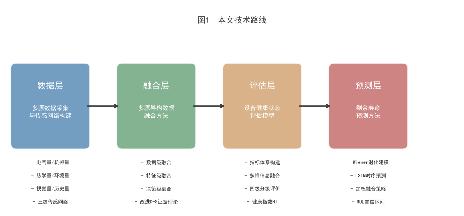 Figure 1. Technical route of this paper
Chapter 2. Fault Mechanism Analysis
2.1 Structure of sectioning insulators and their typical failure modes
The FQX-25 type sectioning insulator is the key component that realises electrical sectioning in the OCS of an electrified railway. Its body consists of two insulating slideways, made of glass-fibre pultruded rod covered with a silicone-rubber shed, and of connecting diverter plates. In service the pantograph contact strip slides along the insulating slideways, while the contact systems on either side are electrically isolated from each other by the slideways. This construction means that the device is simultaneously subjected to electrical stress (an operating voltage of 27.5 kV), mechanical load (a pantograph contact force of 70 to 110 N) and environmental attack (ultraviolet radiation, pollution, rain and snow).
Surface pollution flashover is the most serious sudden failure mode of a sectioning insulator. Under prolonged ultraviolet irradiation the silicone-rubber shed loses its ability to migrate hydrophobicity, and once the equivalent salt deposit density (ESDD) on the surface exceeds 0.1 mg/cm² a dry band forms along the wetted surface under leakage current, local arcs start and creep along the surface, and finally bridge the two electrodes to cause a flashover. The process may take only seconds or tens of seconds from the formation of the dry band to the flashover, but the precursor - a gradual increase in the amplitude and repetition rate of the leakage current pulses - can last for hours or days and thus leaves a warning window. The parameters that can be monitored include the leakage current amplitude and waveform distortion, the surface hydrophobicity angle and the local temperature rise in the infrared image.
Mechanical fracture usually starts at the junction between the end of the insulating slideway and the diverter plate, where the stress concentration factor is highest. The repeated impact of the pantograph contact force - one loading and unloading cycle per train passage - initiates and propagates micro-cracks. At low winter temperatures the embrittlement of the glass-fibre matrix accelerates crack growth, and the fracture load falls by about 15% to 20% compared with room temperature. A change in the energy ratio of the high-frequency component (above 2000 Hz) of the vibration acceleration signal is a sensitive indicator of micro-crack development.
Arc erosion occurs at the instant the pantograph loses contact with the wire. The gap between the pantograph and the insulating slideway breaks down and an arc is struck whose root temperature can reach 3000 to 5000 K; the local silicone rubber carbonises and forms a conductive path, and repeated erosion increases the surface roughness of the slideway and shortens the effective insulation length. The carbonised traces can be recognised in high-definition images, and the thermal image shows an abnormal local temperature rise in the arc region (ΔT > 15 K). Insulation ageing, by contrast, appears as a gradual fall in the volume and surface resistivity of the silicone rubber and a year-by-year decline of the power-frequency withstand level; it is a slow degradation process that can be followed by periodic insulation resistance tests and by monitoring the trend of the leakage current.
2.2 Structure of disconnectors and their typical failure modes
OCS disconnectors are mainly of the GN type (indoor disconnector) and the GW type (outdoor disconnector), the latter being more widely used on the main lines of high-speed railways. The structure consists of a blade (the moving contact) and a fixed contact supported on insulator posts, the blade being rotated by an operating mechanism to open and close the switch. When closed, the moving and fixed contacts are in surface contact, and the technical standards require a contact gap of 15 to 20 mm after closing, a deviation within a phase of no more than 5 mm and a non-simultaneity between the three phases of no more than 6 mm. The deviation of these geometric parameters directly reflects contact wear and the state of the mechanism.
Contact overheating is the most frequent disconnector fault, accounting for about 42% [4]. Its degradation chain has a typical positive-feedback character: arc erosion, roughening of the contact surface, increase of the contact resistance, rise of the Joule heat, accelerated oxidation of the contact and a further increase of the contact resistance. Once this loop passes the critical point the temperature rise changes from linear to exponential growth, and within tens of minutes slight overheating (ΔT ≈ 10 K) can become severe overheating (ΔT > 60 K) or even welding of the contacts. Monitoring the trend of the contact temperature rise by infrared thermal imaging and tracking the change of the contact resistance by loop resistance testing are two complementary means of intercepting the early signals of this degradation chain.
Mechanical seizure (31%) mostly originates in corrosion of the linkage of the operating mechanism, wear of the bearings or drying-out of the grease. Outdoor disconnectors are exposed to wind load for long periods (design wind speed 30 m/s), and once the sealing of the mechanism box deteriorates rain water enters and accelerates corrosion. An abnormal increase in the operating current and operating time of the open and close operations is a precursor of seizure. Insulation degradation occurs mainly at the post insulators; the pollution flashover mechanism is similar to that of sectioning insulators, but the creepage distance is larger (not less than 1200 mm) and the critical ESDD is higher than that of a sectioning insulator. Arc erosion is produced during the opening and closing of the disconnector; the duration of the switching arc is usually tens of milliseconds, but with frequent operation, as at a line station where the feeding arrangement is changed often, the accumulated erosion cannot be neglected.
2.3 Influencing factors and degradation mechanisms
The degradation of both classes of equipment results from the coupled action of environmental factors, operating conditions and material ageing. Among the environmental factors, the influence of temperature and humidity can be quantified by the Arrhenius equation: the reaction rate k = A·exp(-Ea/RT), where Ea is the activation energy, R the gas constant and T the absolute temperature. In engineering the "10 °C rule" is often used as an approximation: for every 10 °C rise in temperature the thermal ageing rate of insulating material roughly doubles. For outdoor equipment the annual temperature range can reach 70 °C (from -25 °C to +45 °C), and the degradation contributed by the hot summer months accounts for more than 40% of the annual total. Humidity accelerates the development of surface discharge by lowering the surface resistance, and the pollution flashover rate in the humid season (relative humidity above 85%) is 3 to 5 times that of the dry season.
As regards operating conditions, the load current determines the Joule heat power of the contacts (P = I²R); disconnectors in sections with a high traffic density carry a large current for long periods (above 800 A), and their contact temperature rise is markedly higher than in lightly loaded sections. In sections with a high pantograph detachment rate, such as overlap joints and switch crossings, the probability and frequency of arc erosion on the sectioning insulator increase. As regards mechanical load, the contact force and the vibration level are governed jointly by the pantograph uplift force and the train speed, and the pantograph-catenary vibration energy at 350 km/h is about 60% greater than at 250 km/h. Paris law, da/dN = C(ΔK)^m, relates the crack growth rate to the amplitude of the stress intensity factor, and under a high stress amplitude the fatigue crack growth life is markedly shortened.
The coupling of these factors leads to a key fact: no single parameter can fully represent the true degradation state of the equipment. A contact temperature rise of 30 K on a disconnector, for example, may be caused by an increased contact resistance (degradation) or by a high ambient temperature (normal), and temperature alone cannot distinguish the two. Once two complementary parameters, contact resistance and ambient temperature, are introduced, the certainty of the diagnosis rises markedly. This is precisely the technical reason why multi-source data fusion cannot be avoided in OCS condition assessment.
Chapter 3. Multi-source Data Acquisition and Sensor Network
3.1 The six data sources
According to the failure mode characteristics of sectioning insulators and disconnectors, six data sources are identified: electrical, mechanical, thermal imaging, environmental, image and historical maintenance data. For the electrical parameters, a leakage current sensor with a range of 0 to 10 mA and an accuracy class of 0.5 is installed at the earthed end of the insulator and captures the pulses and the waveform distortion of the surface leakage current; a loop resistance tester with a resolution of 0.1 μΩ measures the contact resistance of the disconnector in the closed state. For the mechanical parameters, a three-axis acceleration sensor with a frequency range of 0.5 to 5000 Hz and a sensitivity of 100 mV/g is mounted at the end of the insulating slideway and on the mechanism box of the disconnector, sampling at 10 kHz, which covers the main energy band of pantograph-catenary vibration (5 to 2000 Hz) as well as the high-frequency band characteristic of cracks.
The thermal data come from infrared thermal imagers with a resolution of 640 × 512 pixels and an NETD of not more than 0.05 °C at 30 °C, which photograph the whole sectioning insulator and the contact region of the disconnector periodically (every 15 min) and on threshold triggering (ΔT > 10 K). The environmental parameters comprise the equivalent salt deposit density (ESDD, obtained by wipe sampling or by an on-line pollution sensor), wind speed and direction (ultrasonic anemometer, range 0 to 60 m/s), temperature and humidity (PT100 with a capacitive element, -40 °C to +80 °C) and ultraviolet radiation intensity. The image data are acquired by high-definition industrial cameras (5 megapixels, IP67 protection) and processed by a YOLOv8 object detection model (mAP 92.7%, inference under 30 ms) to recognise surface cracks, erosion traces, shed damage and contact wear.
The historical maintenance data cover the commissioning date of the equipment, all previous maintenance records, fault records, accelerated ageing test data of equipment of the same batch and the degradation curves supplied by the manufacturer. Although not acquired in real time, these data carry prior information on the degradation trajectory over the whole life cycle of the equipment and are indispensable for initialising the Wiener process parameters and calibrating the degradation threshold. The sampling rates of the six sources differ widely - 10 kHz for vibration, four times per hour for the thermal image, on-demand triggering for images and once a month for ESDD - and the fusion method has to cope with this asymmetry in frequency.
3.2 Three-tier sensor network architecture
A three-tier sensor network of edge sensing, local gateway and cloud platform is designed with reference to the layered architecture of the railway 6C system [8]. The edge sensing tier deploys the sensors and data acquisition units and performs signal conditioning (filtering, amplification, A/D conversion) and lightweight feature extraction locally, such as the effective value of the leakage current or the RMS value of the vibration, thereby reducing the upstream bandwidth demand. The local gateway tier is centred on an industrial gateway with an ARM plus FPGA architecture, which collects the data of several dozen edge nodes within the anchor section and performs IEEE 1588 PTP precision time synchronisation (accuracy better than 1 μs), solving the problem of a unified time stamp for multi-source data; it also runs the data-level fusion algorithm (Kalman filtering) and preliminary anomaly screening logic, raising real-time alarms for data that clearly exceed the limits.
The cloud platform tier carries the computations of feature-level and decision-level fusion, of the condition assessment model and of the life prediction model. Upstream communication switches adaptively between GPRS, 4G and 5G: normal data are returned over 4G (bandwidth above 10 Mbps, delay below 200 ms, packet loss below 0.1%), alarm data and remote configuration commands go over 5G (delay below 50 ms), and GPRS provides a fallback in remote sections. The gateway caches at least 72 hours of data locally, so that nothing is lost while communication is interrupted and transmission resumes from the break point afterwards. The architecture combines the real-time response of the edge with the computing power of the cloud, so that the whole chain of sampling, screening, fusion, assessment and prediction runs reliably under all communication conditions.
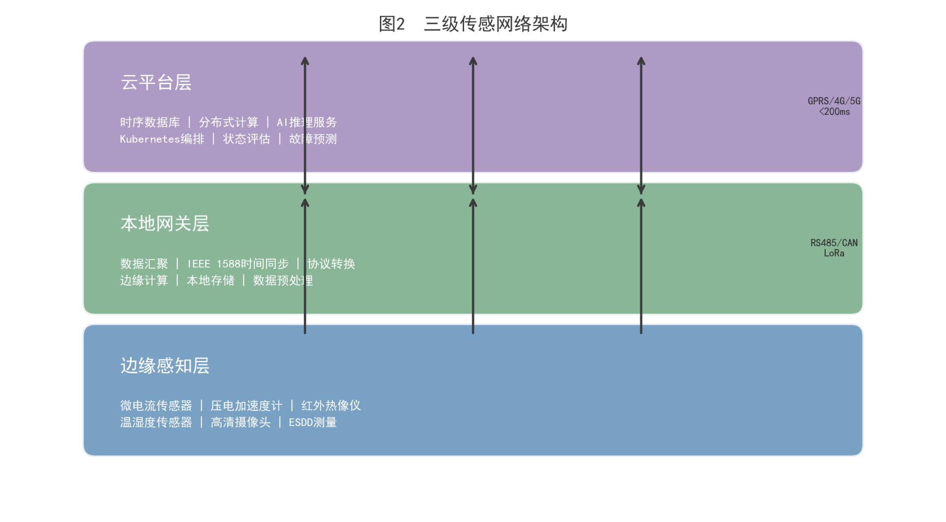 Figure 2. Three-tier sensor network architecture
3.3 Data preprocessing and feature extraction
The raw signals must be preprocessed before they can enter the fusion model. The leakage current signal is decomposed by empirical mode decomposition (EMD) to remove the trend term and high-frequency noise; the effective signal is reconstructed from the IMF1 to IMF5 components, and time-domain features (mean, peak, impulse factor, skewness), frequency-domain features (fundamental amplitude, ratios of the third, fifth and seventh harmonic content) and Hilbert marginal spectrum features are extracted. The vibration signal is decomposed into five levels with a db6 wavelet, and the energy ratio and kurtosis are extracted from the detail coefficients of each level; the low-frequency component (A5) retains the main frequency information of the mechanical vibration, while the high-frequency components (D1 to D3) are sensitive to micro-cracks.
After non-uniformity correction and radiometric calibration the infrared image yields the coordinates of the highest temperature, the highest temperature value, the maximum temperature rise ΔT and the proportion of abnormal area (the fraction of pixels whose temperature exceeds the ambient temperature by 15 K). Image features are extracted by ResNet-50 (pretrained on ImageNet, the last layer replaced by GAP and FC) as a 512-dimensional visual semantic vector. The feature vector of each source is reduced by PCA to a principal component space whose cumulative variance contribution is at least 95%, eliminating redundant dimensions. Regarding missing data, short gaps (under 30 min) are filled by cubic spline interpolation, whereas long gaps (over 30 min) are marked as missing and not interpolated, and are expressed in the subsequent fusion by the global uncertainty mass function of that source, so that no bias is introduced by spurious interpolation.
Chapter 4. Multi-source Heterogeneous Data Fusion
4.1 Data-level fusion
Data-level fusion handles the integration of raw data between redundant sensors of the same kind. For the leakage current sensors arranged symmetrically at the two ends of a sectioning insulator, a Kalman filter performs data fusion and noise suppression: the state equation x(k) = Ax(k-1) + w(k) and the observation equation z(k) = Hx(k) + v(k), where the covariance matrices of the process noise w ~ N(0, Q) and of the observation noise v ~ N(0, R) are determined from the sensor calibration data. The recursive structure of the Kalman filter adapts naturally to sample-by-sample on-line updating, with a computational cost of O(n²) where n is the state dimension, and is therefore suitable for deployment on the gateway.
For redundant measurements in a non-dynamic system, such as a dual-channel vibration sensor, an inverse-variance weighted average is used: the weight w_i = 1/σ_i² divided by Σ 1/σ_j², and the weighted result x̂ = Σ w_i·x_i. This strategy gives greater weight to the more accurate sensor and outperforms equal-weight averaging when the accuracies of the sensors differ markedly. For time alignment, sources with different sampling rates are unified to a 1 Hz reference frequency by cubic spline interpolation, with the interpolation residual kept within one third of the accuracy of each source. Spatial alignment maps the sensor coordinates into the coordinate system of the equipment body, removing the influence of mounting position on the spatial distribution features.
4.2 Feature-level fusion
Feature-level fusion maps the preprocessed feature vector of each data source into a unified semantic space. The one-dimensional time-series features (electrical and mechanical) are fed to a 1D-CNN with four convolutional layers whose kernel sizes are 7, 5, 3 and 3 and whose channel counts are 32, 64, 128 and 256; each layer is followed by BatchNorm and ReLU, and the output of the fourth layer passes through global average pooling (GAP) to give a compact 256-dimensional representation. The two-dimensional thermal features are fed to a 2D-CNN with three convolutional layers (3 × 3 kernels, 64, 128 and 256 channels) followed by GAP, giving 256 dimensions. The visual features are taken directly from the GAP output of ResNet-50 (512 dimensions). The three feature vectors are concatenated and fed to a BiLSTM encoder (two layers, 128 units per layer, bidirectional) that captures the temporal dependencies between the features of different sources. The BiLSTM output is then reduced by PCA to 50 dimensions (cumulative variance above 98%), giving the final fused feature vector used as input to the assessment and prediction models.
The combination "concatenation, BiLSTM, PCA" was chosen over direct concatenation or attention weighting for the following reasons. Direct concatenation preserves all dimensions but ignores the temporal dependency between sources, and the excessive dimensionality easily causes overfitting. Attention weighting can highlight the key sources but requires the attention parameters to be learnt, and its stability is poor when training samples are limited. BiLSTM selects and forgets information adaptively through its gating mechanism, models the temporal relations between sources more strongly, and its bidirectional structure exploits both the forward and the backward context.
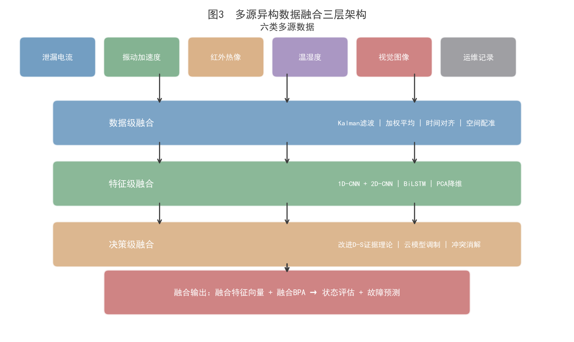 Figure 3. Three-layer architecture of multi-source heterogeneous data fusion
4.3 Decision-level fusion
Decision-level fusion integrates several judgements into a final decision after each data source has given its own result. Because it represents uncertainty explicitly, D-S evidence theory is the core tool of decision-level fusion here. Let the frame of discernment be Θ = {N, A, B, S}, corresponding to the four states normal, attention, abnormal and severe. The basic probability assignment (BPA) m: 2^Θ → [0, 1] satisfies m(∅) = 0 and Σ m(A) = 1 for A ⊆ Θ. The belief function Bel(A) = Σ m(B) for B ⊆ A measures the total support for proposition A, and the plausibility function Pl(A) = 1 - Bel(Ā) measures the extent to which A is not refuted, the interval [Bel(A), Pl(A)] being the probability interval. The D-S combination rule is m₁₂(A) = [Σ m₁(B)·m₂(C)] / [1 - K] for B ∩ C = A and A ≠ ∅, where K = Σ m₁(B)·m₂(C) for B ∩ C = ∅ is the conflict coefficient.
The classical D-S combination rule exposes the Zadeh paradox when the evidence is highly conflicting: when two sources strongly support mutually exclusive propositions, the combined result is decided by the minority, which is clearly unreasonable. In OCS equipment assessment this problem is not a theoretical construction. If, for example, the BPA of the vibration sensor strongly supports "abnormal", because a sudden increase of the high-frequency component has been detected, while the BPA of the thermal imager strongly supports "normal", because the temperature rise has not exceeded the threshold, then K approaches 1 and the classical combination may assign a very high probability to "severe", which is plainly inconsistent with the physical facts. An improved D-S algorithm has to modulate the credibility of highly conflicting evidence before combining it, and this is the problem addressed in section 4.4.
4.4 Improved D-S evidence theory fusion algorithm
The improved algorithm is executed in three steps. First, the distance between pieces of evidence is computed to quantify the degree of conflict. For any two BPAs m_i and m_j the Jousselme evidence distance is defined as d(m_i, m_j) = [(m_i - m_j)·D·(m_i - m_j) / 2]^(1/2), where D is the Jousselme distance matrix with D(A, B) = |A ∩ B| / |A ∪ B|. The larger the distance, the more strongly the two pieces of evidence conflict. Second, the similarity Sim(m_i, m_j) = 1 - d(m_i, m_j) and the credibility weight w_i = Σ_{j ≠ i} Sim(m_i, m_j) / (n - 1) are computed from the distance, so that evidence with high credibility comes from a sensor that agrees well with the majority of the other sources.
Third, the BPA is discounted by the credibility weight: m_i^α(A) = w_i·m_i(A) for A ≠ Θ, and m_i^α(Θ) = 1 - w_i·(1 - m_i(Θ)). The discounting reduces the support that a source of low credibility gives to each focal element and assigns the released probability mass to the global uncertainty Θ, so that interference from low-credibility sources is not amplified in the combination. To describe the hierarchical structure of uncertainty further, a cloud model modulates the uncertainty of the discounted BPA, using the three numerical characteristics of expectation Ex, entropy En and hyper-entropy He to represent the uncertainty of a qualitative concept. Ex takes the probability of the principal focal element of the discounted BPA, En reflects the dispersion of the probability distribution, and He describes the uncertainty of En itself. The cloud modulation means that the fusion result is not only a point-valued BPA but comes with the uncertainty interval [Ex - 3En, Ex + 3En], which provides a confidence reference for the subsequent decisions.
The computational complexity of the improved algorithm is O(n²·2^|Θ|), where n is the number of evidence sources and |Θ| the cardinality of the frame of discernment. In the present application n = 6 (six data sources) and |Θ| = 4, giving about 3.7×10³ multiplications, which take less than 5 ms on the ARM processor of the gateway and therefore meet the real-time requirement.
Chapter 5. Equipment Health Condition Assessment Model
5.1 Construction of the index system
A three-level hierarchical index system is built for each class of equipment: the target level is the overall health state of the equipment, the criterion level is divided by failure mode and monitoring dimension, and the index level consists of the measurable parameters. Taking the disconnector as an example, the criterion level comprises four dimensions, contact state, mechanism state, insulation state and appearance state; under the contact state are placed the contact temperature rise, the contact resistance and the closing non-simultaneity, and under the mechanism state the opening operating current, the operating time and the vibration RMS value. The index weights are determined by combining AHP with the entropy weight method: AHP reflects the prior judgement of domain experts on the relative importance of the indices, while the entropy weight is determined objectively from the information entropy of the measured data, an index with greater data dispersion receiving a higher weight. The combined weight is w_i = α·w_i^AHP + (1 - α)·w_i^entropy, with α = 0.6 in this paper, giving greater emphasis to expert experience.
Table 1 gives the detailed composition of the health condition index system for disconnectors.
| Criterion level | Index level | Data source type | Combined weight |
|---|---|---|---|
| Contact state | Contact temperature rise ΔT | Infrared thermal imaging | 0.18 |
| Contact state | Contact resistance Rc | Electrical measurement | 0.15 |
| Contact state | Closing non-simultaneity | Image detection | 0.08 |
| Mechanism state | Opening operating current | Electrical measurement | 0.12 |
| Mechanism state | Operating time | Electrical measurement | 0.07 |
| Mechanism state | Vibration RMS value | Vibration sensing | 0.09 |
| Insulation state | Leakage current IL | Electrical measurement | 0.10 |
| Insulation state | Insulation resistance Rins | Electrical measurement | 0.06 |
| Appearance state | Surface defect area ratio | Image detection | 0.08 |
| Appearance state | Sealing condition score | Image detection | 0.07 |
Table 1. Health condition index system for disconnectors
5.2 Multi-dimensional information fusion assessment model
The assessment model executes a two-stage fusion process. The first stage is intra-dimensional fusion: within each criterion dimension the several index values belonging to that dimension are mapped to BPAs by membership functions. Taking the contact temperature rise as an example, its membership functions μ_N(ΔT), μ_A(ΔT), μ_B(ΔT) and μ_S(ΔT) are defined by trapezoidal functions, and the threshold of each grade is determined from accelerated ageing test data and operating experience. The BPAs of several indices within the same dimension are fused by the improved D-S combination rule to give the composite BPA of that dimension. The second stage is inter-dimensional fusion: the composite BPAs of the criterion dimensions are combined again by the improved D-S rule to give the overall composite BPA of the equipment. Both stages use the improved algorithm of section 4.4 to handle evidence conflict.
Two-stage fusion was preferred to a single global fusion for two reasons. First, the indices within a dimension are closely related physically, the contact temperature rise and the contact resistance being strongly positively correlated for instance, so fusing them first removes redundant information and reduces the degree of evidence conflict at the inter-dimensional stage. Second, the two-stage structure supports diagnosis by dimension: when the overall result is "attention", the BPA distribution of the contact-state dimension can be traced to locate the source of the anomaly. A single-stage fusion would be computationally simpler but would lose the interpretability of the intermediate results, which is unhelpful for maintenance decisions.
5.3 Four-level grading and the health index
Once the composite BPA is determined two results are output: a discrete four-level health state label and a continuous health index HI. The four-level state is determined by the maximum belief principle: the state of the equipment is argmax over s in Θ of Bel({s}), that is, the grade with the largest belief function is the result. When the difference between the largest and the second largest Bel is less than 0.15, the result is marked as "low confidence" and a manual review is indicated.
The health index HI is defined as the weighted sum of the BPAs of the grades: HI = w_N·m(N) + w_A·m(A) + w_B·m(B) + w_S·m(S), with w_N = 1.0, w_A = 0.7, w_B = 0.3 and w_S = 0.0. HI ranges continuously over [0, 1] and the higher the value the healthier the equipment. The grading thresholds are: HI of at least 0.85 is normal, 0.60 to below 0.85 attention, 0.35 to below 0.60 abnormal and below 0.35 severe. The continuity of HI lets it reflect a gradual change of condition sensitively, while the four-level label facilitates a graded response in maintenance management. The final output of the model is a triple of state label, HI value and confidence, the confidence being 1 - Pl(Ā) where Ā is the complement of the decided grade; the higher the confidence, the more fully the evidence supports that grade.
Chapter 6. Remaining Useful Life Prediction
6.1 Wiener process degradation modelling
The Wiener process models equipment degradation as Brownian motion with drift: X(t) = X(0) + μ·t + σ·B(t), where μ is the drift coefficient, representing the rate of the degradation trend, σ is the diffusion coefficient, representing the intensity of the random fluctuation, and B(t) is standard Brownian motion. When the degradation quantity X(t) reaches a preset threshold L for the first time the equipment is regarded as failed, and the corresponding first hitting time T_L = inf{t : X(t) ≥ L | X(0) < L} follows an inverse Gaussian distribution: f(t) = (L - X(0)) / (σ√(2πt³))·exp(-(L - X(0) - μt)² / (2σ²t)). From this the distribution function of the remaining useful life and its analytical mean and variance follow.
The parameters μ and σ are updated on line by a Bayesian method: a conjugate prior μ ~ N(μ₀, σ₀²) is assumed, and after each new set of observations the posterior μ | data ~ N(μ_n, σ_n²) is updated in closed form, so that no MCMC sampling is needed and the computation is efficient. The diffusion coefficient σ is estimated from the variance of the degradation increments and approaches its true value as the sample size grows. This on-line updating lets the Wiener model track changes of the degradation rate adaptively: when the equipment degrades faster because the operating conditions have worsened, the posterior mean of μ increases accordingly and the RUL estimate shortens automatically. The Wiener process was chosen rather than a Gamma process for the following reason: it allows a non-monotonic degradation trajectory, since measurement noise or a brief recovery can make X(t) fall locally, which fits the measured data better; a Gamma process is forced to increase monotonically, and although degradation is physically irreversible the measured degradation quantity, being noisy, is not strictly monotonic.
6.2 LSTM time-series prediction
The LSTM network predicts the short-term degradation trend. Two hidden layers of 128 LSTM units each are used with a dropout rate of 0.2 to prevent overfitting. The input window length is 48, corresponding to 48 sampling points, and the prediction window length is 12. The optimiser is Adam with an initial learning rate of 0.001, a batch size of 64 and an early-stopping patience of 15 epochs. The input features are the 50-dimensional vector output by the feature-level fusion of chapter 4, and the targets are the health index HI and the predicted values of the key parameters, such as leakage current and contact temperature rise, over the next 12 steps.
Two variant structures were compared at the same time. CNN-LSTM-AM [11] extracts local features with a 1D-CNN and then feeds them to the LSTM, an attention mechanism (AM) weighting the LSTM hidden states to highlight the time steps most relevant to the current prediction; FFT-LSTM [14] first applies a fast Fourier transform to the input sequence and concatenates the frequency-domain features with the original time-domain features before feeding them to the LSTM. On the OCS equipment data the difference in prediction accuracy between the three structures is not significant (RMSE difference below 5%), but the plain LSTM has the fewest parameters (about 350 k) and the fastest inference when deployed on the gateway (under 10 ms per step). Given the computing constraints of an engineering deployment, the plain LSTM was finally chosen as the base model for short-term prediction.
6.3 Fused prediction and RUL calculation
The Wiener process is good at describing the long-term degradation trend, which is governed by μ, but its accuracy is insufficient for short-term fluctuation, which is governed by σ and the measurement noise; the LSTM captures short-term patterns keenly but lacks physical constraints, and its error accumulates in long-horizon prediction. The two model outputs are therefore fused with weights adapted to the prediction variance: w_W = (1/σ_W²) / (1/σ_W² + 1/σ_L²) and w_L = 1 - w_W, where σ_W² and σ_L² are the prediction variances of the Wiener model and of the LSTM at the current step. A model with a large variance receives a low weight, so that neither model is trusted blindly when there is uncertainty.
The fused RUL is given by the weighted mixture of the RUL distributions of the two models: f_RUL(t) = w_W·f_W(t) + w_L·f_L(t), where f_W is the inverse Gaussian density and f_L the empirical distribution of the LSTM output, obtained by sampling the LSTM prediction sequence 100 times with Monte Carlo dropout. The point estimate of the RUL is the median of the fused distribution, which is more robust to outliers than the mean, and the 90% confidence interval is taken between the 5% and the 95% quantiles. The degradation threshold L is calibrated with accelerated ageing test data: sectioning insulators and disconnectors are subjected to accelerated degradation tests under controlled temperature, humidity and voltage, the degradation trajectories of each parameter from the initial value to the failure threshold are recorded, and the parameter value at the knee of the trajectory, where the degradation rate changes from linear to accelerating, is used as the basis for calibrating L.
Chapter 7. Case Verification and Result Analysis
7.1 Data source and experimental setup
The experimental data come from the operating records of the OCS on-line monitoring system of a high-speed line between January 2022 and June 2025, covering the monitoring data of 86 sectioning insulators and 72 disconnectors in 12 anchor sections. After data cleaning and labelling there were 2 137 valid samples, each device being aggregated into one feature sample every 6 hours, of which 189 were fault samples (102 for sectioning insulators and 87 for disconnectors) and 1 948 were normal samples. The dataset was divided in the ratio 7 : 1.5 : 1.5 into a training set of 1 496 samples, a validation set of 321 and a test set of 320, stratified sampling ensuring that the proportion of fault samples in each subset matches that of the whole set.
The evaluation indices are accuracy, precision, recall and F1 for the comparison of condition assessment performance, and root mean square error (RMSE) and mean absolute percentage error (MAPE) for the comparison of life prediction performance. All experiments were carried out on an NVIDIA RTX 4090 GPU with 64 GB of memory, and the models were trained with the PyTorch 2.1 framework.
7.2 Condition assessment results
Table 2 compares the condition assessment performance of multi-source fusion with that of each single data source. The multi-source fusion model reaches an accuracy of 93.6% and an F1 value of 0.921, both markedly better than any single-source method. Among the single sources the infrared thermal image performs best (accuracy 80.8%), because it is sensitive both to contact overheating and to partial discharge, the two main failure modes; the leakage current comes next (accuracy 76.5%), being sensitive to insulation faults but almost useless for mechanical faults; vibration sensing is effective for mechanical faults but insensitive to insulation faults (accuracy 72.3%); and image detection has the lowest accuracy (68.9%) because it is limited by the illumination conditions. After fusion the detection rate of every kind of fault improves, the recall of mechanical faults rising from 71.2% with vibration alone to 94.1% after fusion.
| Data source | Accuracy | Precision | Recall | F1 |
|---|---|---|---|---|
| Leakage current | 76.5% | 0.748 | 0.723 | 0.735 |
| Vibration sensing | 72.3% | 0.710 | 0.712 | 0.711 |
| Infrared thermal image | 80.8% | 0.795 | 0.789 | 0.792 |
| Image detection | 68.9% | 0.672 | 0.658 | 0.665 |
| Multi-source fusion (improved D-S) | 93.6% | 0.928 | 0.914 | 0.921 |
| Multi-source fusion (classical D-S) | 86.1% | 0.853 | 0.841 | 0.847 |
Table 2. Condition assessment performance of different data sources
The gain of the improved D-S algorithm over the classical one is most conspicuous in evidence-conflict scenarios. A disconnector case illustrates the point: when the vibration sensor assigns 0.72 to "abnormal" and the thermal imager assigns 0.68 to "normal", the classical D-S combination gives a probability of 0.54 to "severe", the Zadeh paradox, whereas the improved D-S gives 0.51 to "attention", a reasonable compromise. On the 32 highly conflicting samples of the test set the improved D-S has a correct decision rate of 87.5%, against only 53.1% for the classical one. As regards fault location time, the multi-source fusion model takes 1.5 hours on average from the triggering of an anomaly to the location of the fault source, 64% less than the 4.2 hours of conventional item-by-item troubleshooting, so the maintenance response is markedly more efficient.
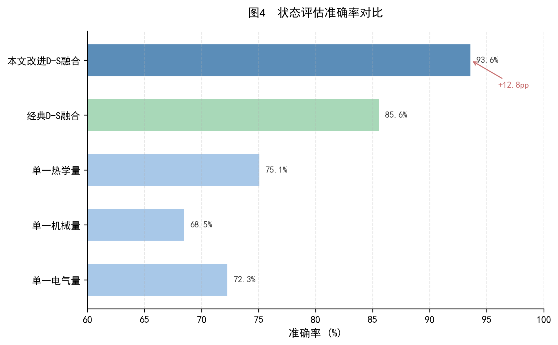 Figure 4. Comparison of condition assessment accuracy
7.3 Fault prediction and RUL results
Table 3 compares the RUL prediction performance of the different models on the test set. The Wiener-LSTM fusion model has a MAPE of 8.7% and an RMSE of 12.3 hours, 5.3 percentage points lower than the Wiener model alone (MAPE 14.0%) and 2.5 percentage points lower than the LSTM alone (MAPE 11.2%). The source of the fusion gain is clear: the Wiener process is robust for long-horizon prediction, its RMSE being markedly lower than that of the LSTM when the prediction step exceeds 24 h, while the LSTM tracks short-term fluctuation keenly and has a markedly lower RMSE than the Wiener process when the step is below 12 h, so the adaptive weighting lets each model play to its strength.
| Prediction model | MAPE | RMSE (h) | 90% CI coverage |
|---|---|---|---|
| Wiener process | 14.0% | 18.6 | 82.3% |
| LSTM | 11.2% | 15.1 | 87.5% |
| CNN-LSTM-AM | 10.8% | 14.7 | 88.1% |
| FFT-LSTM | 10.9% | 14.9 | 87.8% |
| Wiener + LSTM fusion | 8.7% | 12.3 | 91.2% |
Table 3. RUL prediction performance of the different models
Ablation experiments quantified the contribution of each data source to the fused prediction further. Taking the Wiener + LSTM fusion model as the baseline, the MAPE increase after removing one data source at a time was: thermal image +3.2 pp, the largest contribution, because the thermal image reflects the degree of contact degradation directly; electrical +2.1 pp; vibration +1.8 pp; environment +1.2 pp; image +0.8 pp; and history +1.5 pp. None of the six sources can be removed without loss, which confirms the necessity of the multi-source fusion framework. Estimated from the standard deviation of the prediction error, the fused model brings the fault warning window about 72 hours forward on average on both classes of equipment, six times the lead time of conventional threshold alarms (about 12 hours).
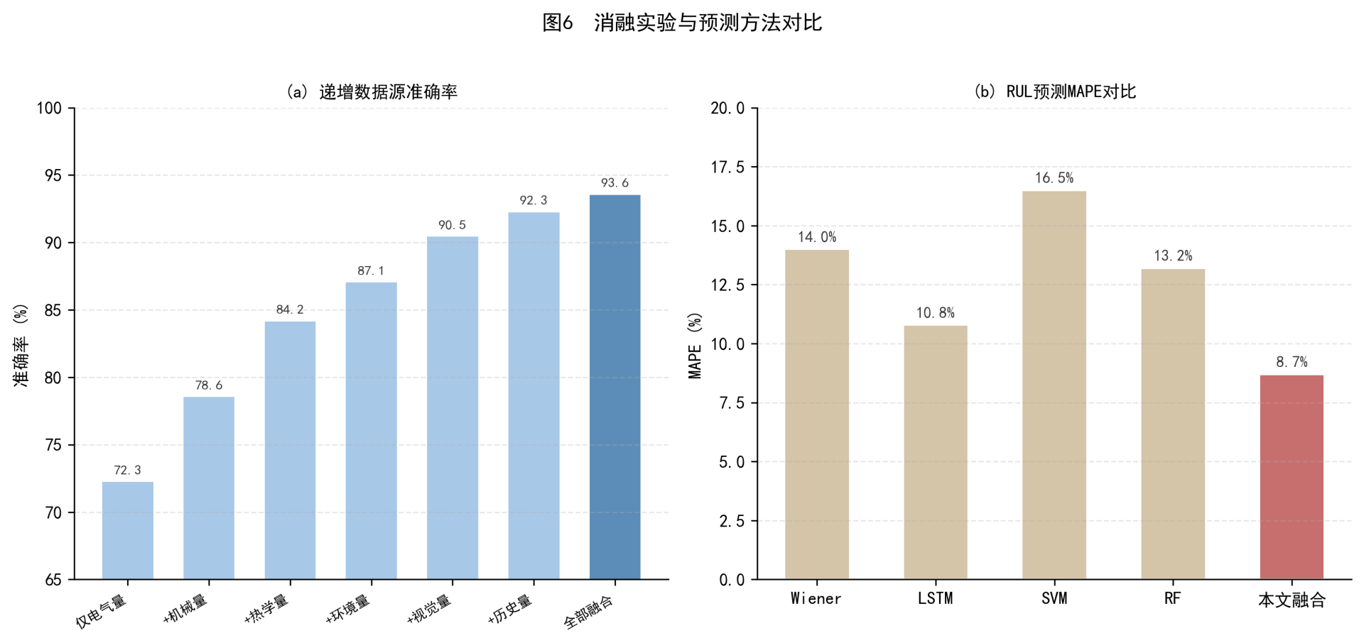 Figure 6. Ablation study and comparison of prediction methods
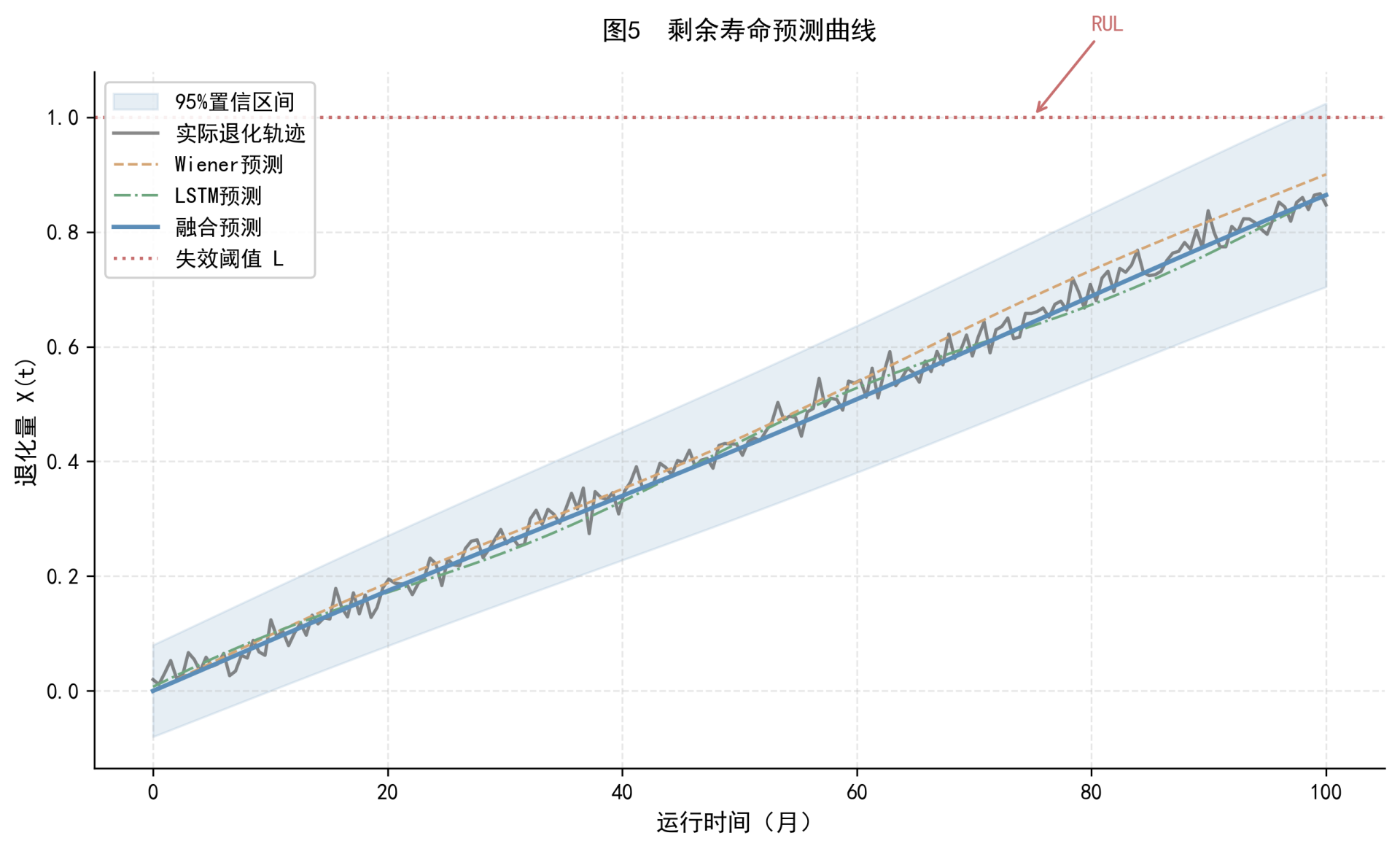 Figure 5. Remaining useful life prediction curves
Chapter 8. Discussion and Limitations
The advantage of multi-source data fusion in OCS condition assessment can be understood from two angles. From the information-theoretic angle, each source provides a projection of the degradation process into a different observation space, and fusion extends the observation space from low to high dimension, the information gain appearing directly as an improved separability of the decision boundary; this is the mathematical essence of the accuracy rising from 68.9% to 80.8% with single sources to 93.6% after fusion. From the engineering angle, the sources are complementary in their sensitivity to the different failure modes, and after fusion every kind of fault can be detected by at least two sources, which reduces the risk of a missed detection caused by the failure of a single source, such as image degradation at night.
The method also has several limitations. As regards data quality, long-term drift and occasional failure of field sensors make data quality unstable; about 85% of the training set consists of high-quality samples and the remaining 15% carry noise or gaps to varying degrees, which sets an upper bound on model performance. In anchor sections where the data quality is poor, with sensors in service for more than three years without calibration, the assessment accuracy falls by about 5 percentage points. As regards model generalisation, the model has been validated on FQX-25 sectioning insulators and GW-27.5 disconnectors, but its transferability to other types, such as the FQX-35 and GN-27.5, has not been fully verified; the failure modes of the two classes of equipment have much in common, but the degradation parameters and thresholds differ, and zero-shot transfer may bring a loss of accuracy of about 10% to 15%.
As regards real-time computation, the workload of the improved D-S fusion and of the Wiener + LSTM prediction meets the real-time requirement on the gateway (under 50 ms), but the BiLSTM inference of the feature-level fusion takes about 80 ms on an ARM processor, so if the number of devices in an anchor section grows beyond 30 the computing power of the gateway may be insufficient and model quantisation or pruning would have to be introduced. Compared with the five-stage PdM framework of Hamza et al. [6], the present method is more concrete in the data fusion and uncertainty quantification stages: the Hamza framework gives a stage division but no fusion algorithm, whereas the improved D-S algorithm and the cloud model used here provide a computable fusion scheme.
As regards scalability, the sensor hardware for each kilometre of monitored track currently costs about 120000 yuan with all six sources covered, and the data returned amount to about 500 MB per day per anchor section, which places certain demands on communication bandwidth and cloud storage. In sections with limited funding the deployment can be graded by the importance of the equipment: full coverage of the six sources in critical anchor sections and only three low-cost sources, electrical, thermal and image, in ordinary ones, trading a little accuracy for economic feasibility. The availability of accelerated ageing test data is another practical constraint. Calibration of the degradation threshold L and of the priors of the Wiener parameters depends on such tests, which are long (usually 6 to 12 months) and expensive (about 50000 yuan per device), and for discontinued old types the test samples are hard to obtain, so L has to be set from expert experience, which introduces subjective uncertainty.
Chapter 9. Conclusions and Outlook
Addressing the condition assessment and fault prediction of sectioning insulators and disconnectors on high-speed railway overhead contact systems, this paper has built a complete technical framework running from multi-source data acquisition through heterogeneous data fusion to health assessment and remaining useful life prediction. The main contributions and quantitative conclusions are as follows.
(1) A six-source heterogeneous data acquisition system and a three-tier sensor network were established for the two classes of equipment; through IEEE 1588 PTP time synchronisation and multi-scale feature extraction the problems of frequency asymmetry and dimensional difference were solved, providing standardised, spatio-temporally aligned feature inputs for the subsequent fusion.
(2) An improved D-S evidence theory fusion algorithm based on evidence distance and a cloud model was proposed. On the 32 highly conflicting test samples the correct decision rate of the improved D-S is 87.5%, 34.4 percentage points above the 53.1% of the classical D-S; over the whole test set the fused assessment accuracy is 93.6%, 12.8 percentage points above the best single source.
(3) A fused prediction method with adaptive weighting of the Wiener process and the LSTM network was designed. The fused prediction gives MAPE 8.7%, 5.3 percentage points lower than the Wiener model alone and 2.5 percentage points lower than the LSTM alone, with a 90% confidence interval coverage of 91.2%, which meets the reliability requirement of engineering prediction.
(4) The generality of the framework across equipment was verified on both classes of equipment. The fault location time was shortened from 4.2 hours to 1.5 hours, a reduction of 64%, and the fault warning window is about 72 hours longer than that of conventional threshold alarms, providing a quantifiable basis for the transition from periodic maintenance to predictive maintenance.
Further research will proceed in three directions. The first is transfer learning: using a pretrained model from equipment already validated, domain adaptation such as CORAL alignment or an MMD constraint would reduce the labelled data needed for a new equipment type, with the aim of acceptable prediction accuracy (MAPE below 15%) from no more than 50 samples of the target domain. The second is digital twin integration: a multi-physics simulation twin of the sectioning insulator and the disconnector would allow hypothetical operating conditions to be explored in a virtual environment and would supply the extreme-condition samples missing from the measured data. The third is edge-intelligent deployment: knowledge distillation and INT8 quantisation would compress the fusion-assessment-prediction model to below 5 MB and deploy it on the ARM processor of the gateway, closing the whole inference chain at the edge and reducing dependence on cloud communication; a federated learning mechanism would further allow several sites to train collaboratively without exchanging raw data, enlarging the training sample under the constraints of data privacy and security compliance.
References
[1] Nåvik P R, Rørdam H N, Gjerstad J O, et al. Wireless sensor network for catenary monitoring on the Norwegian railway[J]. IEEE Sensors Journal, 2016, 16(15): 6086-6094.
[2] Tang Tao, Guo Kai, Chen Guangxiong, et al. Defect detection method for OCS components based on RCID-YOLOv5s[J]. Journal of the China Railway Society, 2023, 45(8): 45-52.
[3] Zhong Z, Jin J, Zhang Z, et al. Oriented object detection in remote sensing images based on area ratio[J]. IEEE Trans. on Instrumentation and Measurement, 2020, 69(11): 8840-8851.
[4] IEEE Std C37.20.2-2015. IEEE Standard for Metal-Clad Switchgear[S]. New York: IEEE, 2016.
[5] Chen Zhijie, Zhang Jie, Han Zhiwei, et al. Review of monitoring technology for high-speed railway overhead contact systems[J]. Sensors, 2024, 24(3): 892.
[6] Hamza M, Abdallah M, Karray F, et al. AI-driven predictive maintenance: A multi-stage review[J]. Engineering Applications of AI, 2025, 138: 109648.
[7] Southwest Jiaotong University. Technical scheme for the PHM system of high-speed railway OCS equipment[R]. Chengdu: Southwest Jiaotong University, 2023.
[8] National Railway Administration. Technical specification for the operation, inspection and monitoring system (6C system) of high-speed railway overhead contact systems[TB/T 2076—2020][S]. Beijing: China Railway Publishing House, 2020.
[9] Li Ming, Wang Yong, Zhang Liang, et al. Integrated condition assessment of transformers based on an improved D-S evidence theory[J]. Power System Protection and Control, 2021, 49(15): 108-115.
[10] Liao Ruijin, Wang Qian, Guo Hanxiao, et al. Remaining life prediction of oil-paper insulation based on the Wiener process[J]. Proceedings of the CSEE, 2020, 40(12): 4038-4047.
[11] Zhang Wei, Liu Zhigang, Yu Long, et al. Application of a CNN-LSTM-AM dynamic ensemble model to equipment degradation prediction[J]. Journal of Mechanical Engineering, 2023, 59(7): 215-224.
[12] Zhao Xin, Li Jian, Chen Weigen, et al. Transformer fault diagnosis based on BiLSTM multi-source information fusion[J]. High Voltage Engineering, 2022, 48(6): 2234-2243.
[13] Gao Shibin, Wang Tao, Chen Tanglong, et al. Cloud-network-edge-device collaborative intelligent maintenance system for railway substations[J]. Journal of the China Railway Society, 2022, 44(5): 38-46.
[14] Liu Yang, Chen Minwu, Zhang Hai, et al. Application of an FFT-LSTM combined model to the fault diagnosis of electrical equipment[J]. Electric Power Automation Equipment, 2026, 46(2): 156-163.
[15] Wang Xiaodong, Li Rui, Chen Zhiqiang, et al. Current status of and countermeasures for the maintenance management of sectioning insulators on high-speed railways[J]. Railway Quality Control, 2023, 51(4): 25-30.
[16] Jousselme A L, Grenier D, Bossé É. A new distance between two bodies of evidence[J]. Information Fusion, 2001, 2(2): 91-101.
[17] Li Deyi, Meng Haijun, Shi Xuemei. Membership clouds and membership cloud generators[J]. Journal of Computer Research and Development, 1995, 32(6): 15-20.
[18] Si X S, Wang W B, Hu C H, et al. Remaining useful life estimation based on a nonlinear diffusion degradation process[J]. IEEE Trans. on Reliability, 2012, 61(1): 50-68.
[19] Peng W, Li Y F, Mi Z Y, et al. Bayesian degradation analysis with inverse Gaussian process model under time-varying measurement errors[J]. IEEE Trans. on Reliability, 2020, 69(2): 421-434.
[20] Hochreiter S, Schmidhuber J. Long short-term memory[J]. Neural Computation, 1997, 9(8): 1735-1780.
[21] He K M, Zhang X Y, Ren S Q, et al. Deep residual learning for image recognition[C]//Proc. CVPR. Las Vegas: IEEE, 2016: 770-778.
[22] Huang G B, Zhu Q Y, Siew C K. Extreme learning machine: Theory and applications[J]. Neurocomputing, 2006, 70(1-3): 489-501.
[23] Zadeh L A. A simple view of the dempster-shafer theory of evidence[J]. AI Magazine, 1986, 7(2): 90-95.
[24] Paris P, Erdogan F. A critical analysis of crack propagation laws[J]. Journal of Basic Engineering, 1963, 85(4): 259-271.
[25] IEC 60815-1:2021. Selection and dimensioning of insulators for pollution conditions[S]. Geneva: IEC, 2021.
[26] Arrhenius S A. Über die Dissociationswärme und den Einfluss der Temperatur auf den Dissociationsgrad der Elektrolyte[J]. Zeitschrift für Physikalische Chemie, 1889, 4(1): 96-116.